Trait Simulation - Ordinal Multinomial Power
Authors: Sarah Ji, Janet Sinsheimer, Kenneth Lange, Hua Zhou
In this notebook we show how to use the TraitSimulation.jl package we illustrate how TraitSimulation.jl can easily simulate traits from genotype data, all within the OpenMendel universe. Operating within this universe brings potential advantages over the available software(s) when needed for downstream analysis or study design. Using just a few calls on the command line to the appropriate packages within the OpenMendel, we demonstrate how to use the OpenMendel code pipeline to construct the genetic model, simulate the trait and find the power for the Ordinal Multinomial Trait.
Background
The ordinal multinomial model is a powerful way to model stages of disease progression. For a disease like diabetes, the monitoring of the disease's progression may be improved based on several different biomarkers detected in the EHR data, such as diabetes diagnostic codes, diabetes medication, hyperglycemia in blood results defined by HbA1c and fasting glucose levels, and presence of diabetes process of care codes. Then these algorithm can better categorize individuals into disease progression categories that relate to how likely they are to have diabetes. This is motivated by the need for early diagnoses and effective intervention techniques. For a detailed review on the published ordinal model, we provide in the references our most recent published paper in Genetic Epidemiology, Ordered multinomial regression for genetic association analysis of ordinal phenotypes at Biobank scale
This software package, TraitSimuliation.jl addresses the need for simulated trait data in genetic analyses. This package generates data sets that will allow researchers to accurately check the validity of programs and to calculate power for their proposed studies. This package gives users the ability to easily simulate phenotypic traits under generalized linear models (GLMs) or variance component models (VCMs) conditional on PLINK formatted genotype data [3]. In addition, we demo customized simulation utilities that accompany specific genetic analysis options in Open-Mendel; for example, ordered, multinomial traits. We demonstrate these simulation utilities on the example dataset described below.
Demonstration
UK Biobank Example Data
The data in this demo is restricted to a subset of individuals of European ancestry excluding first- and second-degree relatives based off of kinship estimates. We filtered samples by 98% genotyping success rate on all chromosomes and SNPs by 99% genotyping success rate. These measures result in n = 185,565 individuals and 470,228 SNPs for analysis. A more detailed description of the data can be found in the references 3 The data from this notebook can be found in the UK Biobank repository under Project ID: 48152 and 15678 at UK Biobank with the permission of UK Biobank.
We will use the OpenMendel package SnpArrays.jl to read in the PLINK formatted data files.
Double check that you are using Julia version 1.0 or higher by checking the machine information
versioninfo()Julia Version 1.3.0
Commit 46ce4d7933 (2019-11-26 06:09 UTC)
Platform Info:
OS: Linux (x86_64-pc-linux-gnu)
CPU: Intel(R) Core(TM) i9-9920X CPU @ 3.50GHz
WORD_SIZE: 64
LIBM: libopenlibm
LLVM: libLLVM-6.0.1 (ORCJIT, skylake)using Plots, DataFrames, LinearAlgebra, StatsFuns, CSV
using SnpArrays, TraitSimulation, GLM, StatsBase, OrdinalMultinomialModelsReading genotype data using SnpArrays
First use SnpArrays.jl to read in the genotype data. We use PLINK formatted data with the same prefixes for the .bim, .fam, .bed files.
SnpArrays is a very useful utility and can do a lot more than just read in the data. More information about all the functionality of SnpArrays can be found at: https://openmendel.github.io/SnpArrays.jl/latest/
As missing genotypes are often due to problems making the calls, the called genotypes at a marker with too much missing genotypes are potentially unreliable. By default, SnpArrays filters to keep only the genotypes with success rates greater than 0.98 and the minimum minor allele frequency to be 0.01. If the user wishes to change the stringency, change the number given in filter according to SnpArrays.
filename = "/mnt/UKBiobank/ukbdata/ordinalanalysis/ukb.plink.filtered"
full_snps = SnpArray(filename * ".bed");
full_snp_data = SnpData(filename)SnpData(people: 185565, snps: 470228,
snp_info:
│ Row │ chromosome │ snpid │ genetic_distance │ position │ allele1 │ allele2 │
│ │ String │ String │ Float64 │ Int64 │ Categorical… │ Categorical… │
├─────┼────────────┼─────────────┼──────────────────┼──────────┼──────────────┼──────────────┤
│ 1 │ 1 │ rs3131972 │ 0.0 │ 752721 │ A │ G │
│ 2 │ 1 │ rs12184325 │ 0.0 │ 754105 │ T │ C │
│ 3 │ 1 │ rs3131962 │ 0.0 │ 756604 │ A │ G │
│ 4 │ 1 │ rs12562034 │ 0.0 │ 768448 │ A │ G │
│ 5 │ 1 │ rs116390263 │ 0.0 │ 772927 │ T │ C │
│ 6 │ 1 │ rs4040617 │ 0.0 │ 779322 │ G │ A │
…,
person_info:
│ Row │ fid │ iid │ father │ mother │ sex │ phenotype │
│ │ Abstract… │ Abstract… │ Abstract… │ Abstract… │ Abstract… │ Abstract… │
├─────┼───────────┼───────────┼───────────┼───────────┼───────────┼───────────┤
│ 1 │ 1000019 │ 1000019 │ 0 │ 0 │ 1 │ -9 │
│ 2 │ 1000078 │ 1000078 │ 0 │ 0 │ 1 │ -9 │
│ 3 │ 1000081 │ 1000081 │ 0 │ 0 │ 1 │ -9 │
│ 4 │ 1000105 │ 1000105 │ 0 │ 0 │ 2 │ -9 │
│ 5 │ 1000112 │ 1000112 │ 0 │ 0 │ 1 │ -9 │
│ 6 │ 1000129 │ 1000129 │ 0 │ 0 │ 1 │ -9 │
…,
srcbed: /mnt/UKBiobank/ukbdata/ordinalanalysis/ukb.plink.filtered.bed
srcbim: /mnt/UKBiobank/ukbdata/ordinalanalysis/ukb.plink.filtered.bim
srcfam: /mnt/UKBiobank/ukbdata/ordinalanalysis/ukb.plink.filtered.fam
)snpid = full_snp_data.snp_info[!, :snpid] # store the snp_info with the snp names
causal_snp_index = findall(x -> x == "rs6603811", snpid)[:] # find the index of the snp of interest by snpid1-element Array{Int64,1}:
174The published hypertension GWAS analysis includes the following covariates: sex, center, age, age2, BMI, and the top ten principal components to adjust for ancestry/relatedness.
causal_snp = @view full_snps[:, causal_snp_index]185565×1 view(::SnpArray, :, [174]) with eltype UInt8:
0x03
0x03
0x03
0x03
0x03
0x03
0x03
0x03
0x03
0x03
0x03
0x03
0x03
⋮
0x03
0x03
0x03
0x02
0x03
0x03
0x03
0x03
0x03
0x03
0x03
0x03maf(causal_snp)1-element Array{Float64,1}:
0.05023244010820205locus = convert(Matrix{Float64}, causal_snp, impute = true)185565×1 Array{Float64,2}:
2.0
2.0
2.0
2.0
2.0
2.0
2.0
2.0
2.0
2.0
2.0
2.0
2.0
⋮
2.0
2.0
2.0
1.0
2.0
2.0
2.0
2.0
2.0
2.0
2.0
2.0Power Calculation
Now we show how to simulate from customized simulation models that accompany specific genetic analysis options in OpenMendel; for example, ordered, multinomial traits and Variance Component Models.
This example illustrates the use of the simulations to generates data sets allowing researchers to accurately check the validity of programs and to calculate power for their proposed studies.
We illustrate this example in three digestable steps:
- The first by simulating genotypes and covariate values representative for our study population.
- Carry over the simulated design matrix from (1) to create the OrderedMultinomialTrait model object.
- Simulate off the OrderedMultinomialTrait model object created in (2) and run the power analyses for the desired significance level.
The published hypertension GWAS analysis includes the following covariates: sex, center, age, age2, BMI, and the top ten principal components to adjust for ancestry/relatedness.
n = length(locus)
published_covariate_data = CSV.read("/mnt/UKBiobank/ukbdata/ordinalanalysis/Covariate_Final.csv")
covariates = published_covariate_data[:, :]
sex = Float64.(covariates[!, :sex])
185565-element Array{Float64,1}:
1.0
1.0
1.0
0.0
1.0
1.0
0.0
0.0
1.0
1.0
0.0
0.0
0.0
⋮
0.0
1.0
0.0
0.0
1.0
1.0
0.0
0.0
0.0
0.0
0.0
1.0β_full =
[0.58
0.022]3-element Array{Float64,1}:
0.58
0.022
0.03γs = collect(0.02:0.005:0.055)8-element Array{Float64,1}:
0.02
0.025
0.03
0.035
0.04
0.045
0.05
0.055X_full = [sex locus]185565×3 Array{Float64,2}:
1.0 1.0 2.0
1.0 1.0 2.0
1.0 1.0 2.0
1.0 0.0 2.0
1.0 1.0 2.0
1.0 1.0 2.0
1.0 0.0 2.0
1.0 0.0 2.0
1.0 1.0 2.0
1.0 1.0 2.0
1.0 0.0 2.0
1.0 0.0 2.0
1.0 0.0 2.0
⋮
1.0 0.0 2.0
1.0 1.0 2.0
1.0 0.0 2.0
1.0 0.0 1.0
1.0 1.0 2.0
1.0 1.0 2.0
1.0 0.0 2.0
1.0 0.0 2.0
1.0 0.0 2.0
1.0 0.0 2.0
1.0 0.0 2.0
1.0 1.0 2.0link = LogitLink()
θ = [1.0, 1.2, 1.4]
Ordinal_Model_Test = OrderedMultinomialTrait(X_full, β_full, θ, link)Ordinal Multinomial Model
* number of fixed effects: 3
* number of ordinal multinomial outcome categories: 4
* link function: LogitLink
* sample size: 185565Now, we can do the same procedure for three snps with different minor allele frequencies, and super impose the power plots to compare the trajectory.
γs = collect(0.0:0.001:0.05)
plot(γs, m22_power, title = "Ordered Multinomial Power", label = "maf = 0.23", lw = 3 , legend = :left, legendfontsize= 9)  # plot power
plot!(γs, m109_power, label = "SNP: rs76601697, maf = 0.11", lw = 3 )  # plot power
plot!(γs, m0_0502_power, label = "maf = 0.05", lw = 3 )  # plot power
xlabel!("Odds Ratio for Associated SNP")
hline!([.8], label = "power = 80%, n = 20,000, alpha = 5*10^-8", lw = 1)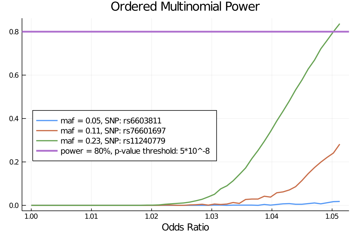
Citations:
[1] Lange K, Papp JC, Sinsheimer JS, Sripracha R, Zhou H, Sobel EM (2013) Mendel: The Swiss army knife of genetic analysis programs. Bioinformatics 29:1568-1570.`
[2] OPENMENDEL: a cooperative programming project for statistical genetics. Hum Genet. 2019 Mar 26. doi: 10.1007/s00439-019-02001-z.
[3] German, CA, Sinsheimer, JS, Klimentidis, YC, Zhou, H, Zhou, JJ. Ordered multinomial regression for genetic association analysis of ordinal phenotypes at Biobank scale. Genetic Epidemiology. 2019; 1– 13. https://doi.org/10.1002/gepi.22276