TraitSimulation.jl
Authors: Sarah Ji, Kenneth Lange, Janet Sinsheimer, Jin Zhou, Hua Zhou, Eric Sobel
We present TraitSimulation, an open-source Julia package that makes it trivial to quickly simulate phenotypes under a variety of genetic architectures. This package is integrated into our larger OpenMendel suite of software tools for easy downstream analyses. Julia was purpose-built for scientific programming and provides tremendous speed and memory efficiency, extensive libraries, and easy access to multi-CPU and GPU hardware and to distributed cloud-based parallelization. It is designed to encourage flexible trait simulation with the standard devices of applied statistics, generalized linear models (GLMs)and generalized linear mixed models (GLMMs).TraitSimulation also accommodates many study designs: unrelateds, sibships, pedigrees, or a mixture of all three.
Background
Statistical geneticists employ simulation to estimate the power of proposed studies, test new analysis tools, and evaluate properties of causal models. Although there are existing trait simulators, there is ample room for modernization of currently available simulation models and computing platforms.For example, most phenotype simulators are limited to Gaussian traits or traits transformable to normality, ignoring qualitative traits and realistic, non-normal trait distributions. Modern computer languages, such as Julia, that accommodate parallelization and cloud-based computing are now mainstream but rarely used inolder applications. To meet the challenges of contemporary big studies, it is nearly imperative for geneticists to adopt new computational tools. Although GPU and Threading capabilities are relatively new and under current development, we explore the potential of these language features and present the results to users who are interested in Julia. Users who wish to play with the prototype GPU code for simulation can find the file in the test folder, but we warn users that the CuArrays package will not install if the proper GPU machinery is not detected.
Demonstration
Example Data
We can use the OpenMendel package SnpArrays.jl to both read in and write out PLINK formatted files. Available in the data directory under the Example_Data section of this package, we use the file "EUR_SUBSET" for the demonstration how to simulate phenotypic traits on PLINK formatted data. For convenience we use the common assumption that the residual covariance among two relatives can be captured by the additive genetic variance times twice the kinship coefficient.
In each simulation model, the user can specify parameters, along with the number of repetitions for each simulation model as desired. By default, the simulation will return the result of a single simulation.
Double check that you are using Julia version 1.0 or higher by checking the machine information
versioninfo()Julia Version 1.4.0
Commit b8e9a9ecc6 (2020-03-21 16:36 UTC)
Platform Info:
OS: macOS (x86_64-apple-darwin18.6.0)
CPU: Intel(R) Core(TM) i7-7700HQ CPU @ 2.80GHz
WORD_SIZE: 64
LIBM: libopenlibm
LLVM: libLLVM-8.0.1 (ORCJIT, skylake)using Random, Plots, DataFrames, LinearAlgebra
using SnpArrays, TraitSimulation, GLM, StatsBase, OrdinalMultinomialModels
Random.seed!(1234);Reading genotype data using SnpArrays
First use SnpArrays.jl to read in the genotype data. We use PLINK formatted data with the same prefixes for the .bim, .fam, .bed files.
SnpArrays is a very useful utility and can do a lot more than just read in the data. More information about all the functionality of SnpArrays can be found at: https://openmendel.github.io/SnpArrays.jl/latest/
As missing genotypes are often due to problems making the calls, the called genotypes at a marker with too much missing genotypes are potentially unreliable. By default, SnpArrays filters to keep only the genotypes with success rates greater than 0.98 and the minimum minor allele frequency to be 0.01. If the user wishes to change the stringency, change the number given in filter according to SnpArrays.
filename = "EUR_subset"
EUR = SnpArray(SnpArrays.datadir(filename * ".bed"));
rowmask, colmask = SnpArrays.filter(EUR)
minor_allele_frequency = maf(EUR);
people, snps = size(EUR)(379, 54051)EUR_data = SnpData(SnpArrays.datadir(filename));Here we will use identify by name, which locus to include, first subset the names of all the loci into a vector called snpid and then call the following command to store our design matrix for the model that includes sex and locus of choice.
bimfile = EUR_data.snp_info # store the snp_info with the snp names

snpid  = bimfile[!, :snpid] # store the snp names in the snpid vector

causal_snp_index = findall(x -> x == "rs150018646", snpid) # find the index of the snp of interest by snpid
1-element Array{Int64,1}:
82Additionally, we will control for sex, with females as the baseline group, sex = 0.0. We want to find the index of this causal locus in the snp_definition (.bim) file and then subset that locus from the genetic marker data above. Make note of julia's ternary operator '?' which allows us to make this conversion efficiently!
Using SnpArrays.jl we can then use the convert and @view commands to get the appropriate conversion from SnpArray to a computable vector of Float64.
locus = convert(Vector{Float64}, @view(EUR[:, causal_snp_index[1]]))
famfile = EUR_data.person_info
sex = map(x -> strip(x) == "F" ? 0.0 : 1.0, famfile[!, :sex])
intercept = ones(length(sex))
X_covar = [intercept sex]
X = [intercept sex locus]
379×3 Array{Float64,2}:
1.0 1.0 2.0
1.0 1.0 1.0
1.0 1.0 2.0
1.0 1.0 2.0
1.0 1.0 2.0
1.0 1.0 2.0
1.0 1.0 2.0
1.0 1.0 2.0
1.0 1.0 2.0
1.0 1.0 2.0
1.0 1.0 2.0
1.0 1.0 2.0
1.0 1.0 2.0
⋮
1.0 1.0 2.0
1.0 1.0 2.0
1.0 1.0 1.0
1.0 1.0 2.0
1.0 1.0 2.0
1.0 1.0 2.0
1.0 1.0 2.0
1.0 1.0 2.0
1.0 1.0 2.0
1.0 1.0 2.0
1.0 1.0 2.0
1.0 1.0 2.0Example 1: GLM Trait
In this example we first demonstrate how to use the GLM.jl package to simulate a trait from unrelated individuals. We specify the fixed effects and the phenotype distribution, and output the simulation results.
\[Y \sim Poisson(\mu = g^{-1}(XB))\]
A more thorough application of this GLM TraitSimulation applied to an Iterative Hard Thresholding problem under MendelIHT can be found here:
GLM Traits from Unrelated Individuals
$ Y{n \times 1} \sim Poisson(\mu{n \times 1} = X\beta)$
β = [1; 0.2; 0.5]
dist = Poisson()
link = LogLink()
GLMmodel = GLMTrait(X, β, dist, link)
Generalized Linear Model
* response distribution: Poisson
* link function: LogLink
* sample size: 379 * fixed effects: 3Simulated_GLM_Traits = simulate(GLMmodel)379-element Array{Int64,1}:
4
8
7
10
10
11
7
9
8
9
6
9
10
⋮
7
11
5
11
9
7
5
8
4
12
16
10Example 2: VCM Trait
In this example we show how to generate data so that the related individuals have correlated trait values even after we account for the effect of a snp, a combination of snps or other fixed effects. We simulate data under a variance component model so that we can model residual dependency among individuals.
We note models with additional variance components can also be specified, as long as they are sensible (positive semi definite).
VCMTrait UK Biobank Demo:
For the univariate and bivariate Variance Component Model, we include in the Real Data Examples section our step-by-step procedure of simultaneously simulating and fitting to get the genetic power.
\[Y \sim N(\mu, 4* 2GRM + 2*I_n)\]
\[Y \sim N(\mathbf{\mu}, \sigma_a \otimes 2GRM + \sigma_e \otimes I_n)\]
where we can calculate the estimated empirical kinship matrix $2*\hat{\Phi}_{GRM}$ using SnpArrays.jl. Due to privacy of the data, we include only the html file for viewing.
- Trait Simulation - Variance Component Model Power (UKBiobank)
- Reading genotype data using SnpArrays
- Construct Genetic Model: (VCM Parameter Specification)
- Power Calculation
- Univariate VCM Power
- Bivariate VCM Power
We include some other variance component model examples for family data as follows:
Rare Variant VCM Related Individuals
In this example we show how to generate data so that the related individuals have correlated trait values even after we account for the effect of a snp, a combination of snps or other fixed effects. We simulate data under a linear mixed model so that we can model residual dependency among individuals.
\[Y \sim \text{Normal}(\mathbf{\mu}_{n \times 1} = X\beta, \Sigma_{n \times n} = \sigma_A \times 2\hat{\Phi}_{GRM} + \sigma_E \times I_n)\]
This example is meant to simulate data in a scenario in which a number of rare mutations in a single gene can change a trait value. We model the residual variation among relatives with the additive genetic variance component and we include 20 simulated rare variants in the mean portion of the model, defined as loci with minor allele frequencies greater than 0.002 but less than 0.02.
Specifically we are generating a single normal trait controlling for family structure with residual heritabiity of 67%, and effect sizes for the variants generated as a function of the minor allele frequencies. The rarer the variant the greater its effect size.
In practice rare variants have smaller minor allele frequencies, but we are limited in this tutorial by the relatively small size of the data set. Note also that our modeling these effects as part of the mean is not meant to imply that the best way to detect them would be a standard association analysis. Instead we recommend a burden or SKAT test.
GRM = grm(EUR, minmaf = 0.05);Genotype Simulation:
Say our study population has a sample size of n people and we are interested in studying the effect of the causal snp with a predetermined minor allele frequency. We use the minor allele frequency of the causal variant to simulate the SnpArray under Hardy Weinberg Equillibrium (HWE), using the snparray_simulation function as follows:
| Genotype | Plink/SnpArray |
|---|---|
| A1,A1 | 0x00 |
| missing | 0x01 |
| A1,A2 | 0x02 |
| A2,A2 | 0x03 |
Given a vector of minor allele frequencies, specify maf = [0.2, 0.25, 0.3], for each specified allele it will simulate a SnpArray under HWE and ouput them together. This function samples from the genotype vector under HWE and returns the compressed binary format under SnpArrays.
maf_rare = rand([0.002, 0.004, 0.008, 0.01, 0.012, 0.015, 0.02], 20)
rare_snps = snparray_simulation(maf_rare, 379)
379×20 SnpArray:
0x00 0x00 0x00 0x00 0x00 0x00 … 0x00 0x00 0x00 0x00 0x00 0x00
0x00 0x00 0x00 0x00 0x00 0x00 0x00 0x00 0x00 0x00 0x00 0x00
0x00 0x00 0x00 0x00 0x00 0x00 0x00 0x00 0x00 0x00 0x00 0x00
0x00 0x00 0x00 0x00 0x00 0x00 0x00 0x00 0x00 0x00 0x00 0x00
0x00 0x00 0x00 0x00 0x00 0x00 0x00 0x00 0x00 0x00 0x00 0x00
0x00 0x00 0x00 0x00 0x00 0x00 … 0x00 0x00 0x00 0x00 0x00 0x00
0x00 0x00 0x00 0x00 0x00 0x00 0x00 0x00 0x00 0x00 0x00 0x00
0x00 0x00 0x00 0x00 0x00 0x00 0x00 0x00 0x00 0x00 0x00 0x00
⋮ ⋮ ⋱ ⋮
0x00 0x00 0x00 0x00 0x00 0x00 0x00 0x00 0x00 0x00 0x00 0x00
0x00 0x00 0x00 0x00 0x00 0x00 0x00 0x00 0x00 0x00 0x00 0x00
0x00 0x00 0x00 0x00 0x00 0x00 0x00 0x00 0x00 0x00 0x00 0x00
0x00 0x00 0x00 0x00 0x00 0x00 … 0x00 0x00 0x00 0x00 0x00 0x00
0x00 0x00 0x00 0x00 0x00 0x00 0x00 0x00 0x00 0x00 0x00 0x00
0x00 0x00 0x00 0x00 0x00 0x00 0x00 0x00 0x00 0x00 0x00 0x00
0x00 0x00 0x02 0x00 0x00 0x00 0x00 0x00 0x00 0x00 0x00 0x00
0x02 0x00 0x00 0x00 0x00 0x00 0x00 0x00 0x00 0x00 0x00 0x00
0x00 0x00 0x00 0x00 0x00 0x00 … 0x00 0x00 0x00 0x00 0x00 0x00
0x00 0x00 0x00 0x02 0x00 0x00 0x00 0x00 0x00 0x00 0x00 0x00
0x00 0x00 0x00 0x00 0x00 0x00 0x00 0x00 0x00 0x00 0x00 0x00
0x00 0x00 0x00 0x00 0x00 0x00 0x02 0x00 0x00 0x00 0x00 0x00β_covar = [1.0; 0.6]
I_n = Matrix{Float64}(I, size(GRM))
vc = @vc [0.01][:,:] ⊗ (GRM + I_n) + [0.9][:, :] ⊗ I_n
sigma, v = vcobjtuple(vc)
rare_20_snp_model = VCMTrait(X_covar, β_covar[:, :], rare_snps, maf_rare[:, :], [sigma...], [v...])Variance Component Model
* number of traits: 1
* number of variance components: 2
* sample size: 379Rare_SNP_Trait = simulate(rare_20_snp_model)379×1 Array{Float64,2}:
0.8088744352540489
1.6701367617702745
1.8455248160731537
0.8508388343337788
0.9712931279208524
0.6887865756651992
2.9436570129936905
1.808457300723279
1.1133732340741647
1.0798778322598372
0.8779238588613009
2.338615502643955
3.392334665830318
⋮
3.654119285594163
1.4716923062049176
1.7276952768730827
1.3970739033596746
1.4755462272829616
2.981506123686394
1.6977542002518275
3.09839068211269
3.225180822413689
2.7490032145653913
3.8705735842017255
2.7194612533505413Multiple Traits, Multiple Variance Components? Easy.
This example extends the variance component model in the previous example to demo how to efficiently account for any number of other random effects, in addition to the additive genetic and environmental variance components.
Y ~ MatrixNormal($M = XB$, $Omega = \sum_{k=1}^m \Sigma_{k}$ $\otimes V_k$)
We note that this form can also accompany more than 2 variance components.
I encourage for those interested, to look at this example where we demonstrate the simlation of $d = 2$ traits with $m = 10$ variance components, and benchmark it against the available method using the MatrixNormal distribution in Julia package, Distributions.jl.
Example 3: Ordered Multinomial Trait
Now we demonstrate on the OrderedMultinomialTrait model object in TraitSimulation.jl.
Ordered Multinomial Trait
Recall that this phenotype is special, in that the OrdinalMultinomialModels package provides Julia utilities to fit ordered multinomial models, including proportional odds model and ordered Probit model as special cases.
For this model, we have intercept parameters $\theta_1 \le \cdots \le \theta_{J-1}$ enforce the order between the categories and $\boldsymbol{\beta}$ reflects the effects of the linear predictors under the proportional hazards model. The effect sizes can be interpreted as the expected change of the response variable on an ordered log-odds scale for each unit increase in the predictor.
θ = [1.0, 1.2, 1.4]
Ordinal_Model = OrderedMultinomialTrait(X, β, θ, LogitLink())
Ordinal Multinomial Model
* number of fixed effects: 3
* number of ordinal multinomial outcome categories: 4
* link function: LogitLink
* sample size: 379Ordinal_Trait = simulate(Ordinal_Model)379-element Array{Int64,1}:
2
4
4
1
1
1
1
4
1
4
4
3
4
⋮
4
4
2
1
1
4
1
4
4
4
4
4Simulate Ordered Multinomial Logistic
Specific to the Ordered Multinomial Logistic model is the option to transform the multinomial outcome (i.e 1, 2, 3, 4) into a binary outcome for logistic regression.
Although by default is the multinomial simulation above, the user can simulate from the transformed logistic outcome for example by specifying arguments: Logistic = true and threshold = 2 the value to use as a cutoff for identifying cases and controls. (i.e if y > 2 => y_logit == 1). We note if you specify Logistic = true and do not provide a threshold value, the function will throw an error to remind you to specify one.
Logistic_Trait = simulate(Ordinal_Model, Logistic = true, threshold = 2)379-element Array{Int64,1}:
1
1
1
1
1
1
0
0
1
1
1
0
1
⋮
1
1
0
1
1
1
0
0
1
1
1
1Example 4: GLMM Trait Simulation
Next, we demonstrate how to simulate a Poisson Trait, after controlling for family structure.
dist = Poisson()
link = LogLink()

vc = @vc [0.01][:,:] ⊗ (GRM + I_n) + [0.9][:, :] ⊗ I_n
GLMMmodel = GLMMTrait(X, β[:,:], vc, dist, link)
Generalized Linear Mixed Model
* response distribution: Poisson
* link function: LogLink
* number of variance components: 2
* sample size: 379Y = simulate(GLMMmodel)379×1 Array{Int64,2}:
31
3
5
4
9
10
3
10
17
6
16
24
16
⋮
18
3
4
2
28
5
1
6
32
0
9
13Power Calculation
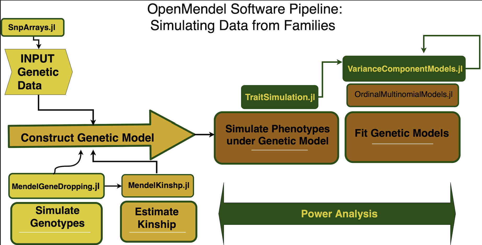
Now we demonstrate the use of the simulations to generates data sets allowing researchers to accurately check the validity of programs and to calculate power for their proposed studies. For these examples we will demo the full power pipeline contained within the OpenMendel environment.
We illustrate this example in three digestable steps as shown in the figure:
- The first by simulating genotypes and covariate values representative for our study population.
- Carry over the simulated design matrix from (1) to create the OrderedMultinomialTrait model object.
- Simulate off the OrderedMultinomialTrait model object created in (2) and run the power analyses for the desired significance level.
Each column of this matrix represents each of the detected effect sizes, and each row of this matrix represents each simulation for that effect size. The user feeds into the function the number of simulations, the vector of effect sizes, the TraitSimulation.jl model object, and the random seed.
\[\mathbf{Y}_{n \times 1} = \mathbf{X}\mathbf{\beta} + \mathbf{G}_s \gamma + \mathbf{g} + \mathbf{\epsilon}\]
\[\mathbf{g} \sim N(\mathbf{0}, \sigma_A \times \mathbf{\Phi})\]
\[\mathbf{\epsilon} \sim N(\mathbf{0}, \sigma_E \times \mathbf{I_n})\]
Here $\sigma_A$ and $\Sigma_A$ are the additive genetic variance and matrix, $\sigma_E$ and $\Sigma_E$ are the environmental variance and matrix, $\mathbf{\Phi}$ is the kinship matrix, and $\mathbf{I_n}$ is the $n \times n$ identity matrix.
We illustrate the example on simulated data under the Ordered Multinomial Model and define the study power in the following way. For each simulated trait, we perform a likelihood ratio test of the above hypothesis test and reject the null when the p-value falls below prespecified significance level. In our example, we define the power for the model is estimated as the proportion of tests rejecting the null at significance level α = 5×10⁻⁸.
\[\textbf{H}_0: \gamma = 0 \hspace{0.25in}\text{versus}\hspace{0.25in} \textbf{H}_A: \gamma \neq 0\]
For GLMTrait objects, the realistic_power_simulation function makes the appropriate calls to the GLM.jl package to get the simulation p-values obtained from testing the significance of the causal locus using the Wald Test by default. However since the GLM.jl package has its limitations, we include additional power utilities that make the appropriate function calls to the OrdinalMultinomialModels to get the p-value obtained from testing the significance of the causal locus. Variance Component Models for VCMTrait objects can be fit using VarianceComponentModels.jl, and we demo for UK Biobank data in the docs.
Guidelines to the UKBiobank Data
The data used in the analysis examples in this manuscript are from the UK Biobank data repository and are publicly available, after approval by their review board, from the UKBiobank. We retrieved the data under Project IDs 48152 and 15678.
UKBiobank Power Pipeline
- Trait Simulation - Variance Component Model Power (UKBiobank)
- Reading genotype data using SnpArrays
- Construct Genetic Model: (VCM Parameter Specification)
- Power Calculation
- Univariate VCM Power
- Bivariate VCM Power
- Trait Simulation - Ordinal Multinomial Power
- Reading genotype data using SnpArrays
- Power Calculation
For each effect size in $\gamma_s,$ in each column we have the p-values obtained from testing the significance of the causal locus nsim = 1000 times under the desired model, and the randomseed = 1234.
Citations:
[1] Lange K, Papp JC, Sinsheimer JS, Sripracha R, Zhou H, Sobel EM (2013) Mendel: The Swiss army knife of genetic analysis programs. Bioinformatics 29:1568-1570.`
[2] OPENMENDEL: a cooperative programming project for statistical genetics. Hum Genet. 2019 Mar 26. doi: 10.1007/s00439-019-02001-z.
[3] German, CA, Sinsheimer, JS, Klimentidis, YC, Zhou, H, Zhou, JJ. Ordered multinomial regression for genetic association analysis of ordinal phenotypes at Biobank scale. Genetic Epidemiology. 2019; 1– 13. https://doi.org/10.1002/gepi.22276