WiSER.jl Introduction
WiSER.jl implements a regression method for modeling the within-subject variability of a longitudinal measurement. It stands for within-subject variance estimation by robust regression.
This package requires Julia v1.0 or later, which can be obtained from https://julialang.org/downloads/ or by building Julia from the sources in the https://github.com/JuliaLang/julia repository.
The package has not yet been registered and must be installed using the repository location. Start Julia and use the ] key to switch to the package manager REPL
(@v1.5) Pkg> add https://github.com/OpenMendel/WiSER.jlUse the backspace key to return to the Julia REPL.
Model
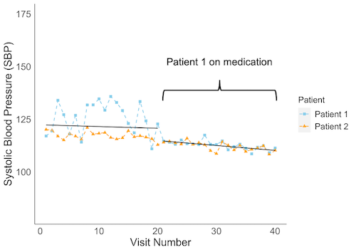
WiSER was created to efficiently estimate effects of covarariates on within-subject (WS) variability in logitudinal data. The following graphic depicts the motiviation for WiSER and what it can model.

The figure above displays systolic blood pressure (SBP) measured for two patients followed up over 40-visits. At baseline, we see a difference in both mean and variability of SBP between the two patients. After the 20th visit, patient 1 goes on blood pressure medication and their mean and WS variance of SBP more similarly match patient 2's. It can be of clinical importance to model what factors associated with these baseline differences in mean and WS variance as well as how being on medication (a time-varying covariate) affects these measures. WiSER is able to simultaneously model (time-invariant and time-varying) covariates' effects on mean and within-subject variability of longitudinal traits.
The mean fixed effects are estimated in $\boldsymbol{\beta}$, the within-subject variance fixed effects are estimated by $\boldsymbol{\tau}$, and the random effects covariance matrix is estimated in $\boldsymbol{\Sigma}_{\boldsymbol{\gamma}}$.
Model Details
In addition to mean levels, it can be important to model factors influencing within-subject variability of longitudinal outcomes. We utilize a modified linear mixed effects model that allows for within-subject variability to be modeled through covariates. It is motivated by a Mixed Effects Multiple Location Scale Model introduced by Dzubar et al. (2020), but WiSER dispenses with the normal assumptions and is much faster than the likelihood method implemented in the MixWILD software.
The procedure assumes the following model for the data:
Data:
- $y_{ij}$ longitudinal response of subject $i$ at time $j$
- $\textbf{x}_{ij}$ mean fixed effects covariates of subject $i$ at time $j$
- $\textbf{z}_{ij}$ random (location) effects covariates of subject $i$ at time $j$
- $\textbf{w}_{ij}$ within-subject variance fixed effects covariates of subject $i$ at time $j$
Parameters:
- $\boldsymbol{\beta}$ mean fixed effects
- $\boldsymbol{\tau}$ within-subject variance fixed effects
- $\boldsymbol{\boldsymbol{\gamma}_i}$ random location effects of subject $i$
- $\boldsymbol{\Sigma}_{\boldsymbol{\gamma}}$ random (location) effects covariance matrix
- $\omega_i$ random scale effect of subject $i$
- $\sigma_\omega^2$ variance of random scale effect
- $\boldsymbol{\Sigma}_{\boldsymbol{\gamma} \omega}$ joint random effects covariance matrix
Other:
- $\mathcal{D(a, b)}$ unspecified distribution with mean $a$ and variance $b$
- $\epsilon_{ij}$ error term of subject $i$ and time $j$ capturing within-subject variability
The longitduinal data are modeled via:
\[\begin{aligned} y_{ij} &=& \textbf{x}_{ij}^T\boldsymbol{\beta} + \textbf{z}_{ij}^T\boldsymbol{\gamma}_i + \epsilon_{ij}, \quad \epsilon_{ij} \sim \mathcal{D}(0, \sigma_{\epsilon_{ij}}^2), \\ \boldsymbol{\gamma_i} &=& (\gamma_{i1}, \gamma_{i2}, \cdots, \gamma_{iq})^T \sim \mathcal{D}(\mathbf{0}_{q}, \boldsymbol{\Sigma}_{\boldsymbol{\gamma}}), \end{aligned}\]
where
\[\begin{aligned} \sigma_{\epsilon_{ij}}^2 = \exp (\textbf{w}_{ij}^T \boldsymbol{\tau} + \boldsymbol{\ell}_{\boldsymbol{\gamma} \omega}^T \boldsymbol{\gamma_i} + \omega_i), \quad \omega_i \sim \mathcal{D}(0, \sigma_\omega^2) \end{aligned}\]
represents the within-subject variance with $\boldsymbol{\ell}_{\gamma \omega}^T$ coming from the Cholesky factor of the covariance matrix of the joint distribution of random effects ($\boldsymbol{\gamma}_i$, $\omega_i$). The joint distribution of random effects is
\[\begin{aligned} \begin{pmatrix} \boldsymbol{\gamma_i} \\ \omega_i \end{pmatrix} \sim \mathcal{D}(\mathbf{0}_{q+1}, \boldsymbol{\Sigma}_{\boldsymbol{\gamma} \omega}) \end{aligned}\]
and denote the Cholesky decomposition of the covariance matrix $\boldsymbol{\Sigma_{\gamma w}}$ as
\[\begin{aligned} \boldsymbol{\Sigma}_{\boldsymbol{\gamma} \omega} &=& \begin{pmatrix} \boldsymbol{\Sigma}_{\boldsymbol{\gamma}} & \boldsymbol{\sigma}_{\boldsymbol{\gamma} \omega} \\ \boldsymbol{\sigma}_{\boldsymbol{\gamma} \omega}^T & \sigma_\omega^2 \end{pmatrix} = \textbf{L} \textbf{L}^T, \quad \textbf{L} = \begin{pmatrix} \textbf{L}_{\boldsymbol{\gamma}} & \mathbf{0} \\ \boldsymbol{\ell}_{\boldsymbol{\gamma} \omega}^T & \ell_{\omega} \end{pmatrix}, \end{aligned}\]
where $\textbf{L}_{\boldsymbol{\gamma}}$ is a $q \times q$ upper triangular matrix with positive diagonal entries and $\ell_{\omega} > 0$. The elements of $\boldsymbol{\Sigma}_{\boldsymbol{\gamma} \omega}$ can be expressed in terms of the Cholesky factors as:
\[\begin{aligned} \boldsymbol{\Sigma}_{\boldsymbol{\gamma}} &=& \textbf{L}_{\boldsymbol{\gamma}} \textbf{L}_{\boldsymbol{\gamma}}^T \\ \boldsymbol{\sigma}_{\boldsymbol{\gamma} \omega} &=& \textbf{L}_{\boldsymbol{\gamma}} \boldsymbol{\ell}_{\boldsymbol{\gamma} \omega} \\ \sigma_\omega^2 &=& \boldsymbol{\ell}_{\boldsymbol{\gamma} \omega}^T \boldsymbol{\ell}_{\boldsymbol{\gamma} \omega} + \ell_{\omega}^2 \end{aligned}\]
In Dzubuar et al's estimation, they assume all unspecified distributions above are Normal distributions. Our estimation procedure is robust and only needs that the mean and variance of those random variables hold. In their MixWILD software, they fit the model through maximum likelihood, requiring numerically intensive numerical integration.
We have derived a computationally efficient and statistically robust method for obtaining estimates of $\boldsymbol{\beta}, \boldsymbol{\tau}, \text{and}, \boldsymbol{\Sigma_\gamma}$. The mean fixed effects $\boldsymbol{\beta}$ are estimated by weighted least squares, while the variance components $\boldsymbol{\tau}$ and $\boldsymbol{\Sigma_\gamma}$ are estimated via a weighted nonlinear least squares approach motivated by the method of moments. WiSER does not estimate any parameters associated with the random scale effect $\omega_i$ or any association between $\boldsymbol{\gamma}_i$ and $\omega_i$. These are treated as nuissance parameters that get absorbed into the intercept of $\boldsymbol{\tau}$.
NOTE: When the true data has a random scale effect with non-zero variance $\sigma^2_\omega$, WiSER's estimates of $\boldsymbol{\beta}$, non-intercept values of $\boldsymbol{\tau}$, and $\boldsymbol{\Sigma_\gamma}$ are consistent. In this case, the intercept of $\boldsymbol{\tau}$ absorbs effects from $\sigma^2_\omega$.