Estimating ancestry

If samples in the reference haplotype panel are labeled with a population origin, MendelImpute can also be used for:

• Local ancestry inference (chromosome painting)
• Global ancestry inference

# first load all necessary packages
using MendelImpute
using StatsPlots

Prepare Example data for illustration

We use the 1000 genomes chromosome 22 as illustration. The original data is filtered into target and reference panels. Follow detailed example in Phasing and Imputation to obtain the same data.

Process each sample's population origin

MendelImpute needs to know each reference sample's origin (country/ethnicity/region...etc). This origin information should be provided by the reference haplotype panel, but users are free to further organize origin labels base on their own criteria. For this purpose, MendelImpute needs a Dict{key, value} where each key is a reference sample ID and the value is the population code. Example dictionaries for 1000 genome project can be created by MendelImpute's internal helper functions. Users not using 1000 genomes would have to manually construct such a dictionary mapping reference sample IDs to a desired population label.

Here is a dictionary mapping sample IDs (from 1000 genomes project) to their super population codes.

refID_to_superpopulation = thousand_genome_samples_to_super_population()

Dict{String, String} with 2504 entries:
  "HG01791" => "EUR"
  "HG02736" => "SAS"
  "HG00182" => "EUR"
  "HG03914" => "SAS"
  "HG00149" => "EUR"
  "NA12156" => "EUR"
  "HG02642" => "AFR"
  "HG02851" => "AFR"
  "NA19835" => "AFR"
  "NA19019" => "AFR"
  "HG01131" => "AMR"
  "HG03578" => "AFR"
  "NA18550" => "EAS"
  "HG02401" => "EAS"
  "HG01350" => "AMR"
  "HG03973" => "SAS"
  "NA07000" => "EUR"
  "HG01709" => "EUR"
  "HG01395" => "AMR"
  "HG01980" => "AMR"
  "HG01979" => "AMR"
  "HG01122" => "AMR"
  "HG03869" => "SAS"
  "HG03729" => "SAS"
  "NA19920" => "AFR"
  ⋮         => ⋮

Here is another dictionary mapping population code to super population codes. Thus we can map samples to super populations.

pop_to_superpop = thousand_genome_population_to_superpopulation()

Dict{String, String} with 26 entries:
  "CHS" => "EAS"
  "CDX" => "EAS"
  "GIH" => "SAS"
  "MSL" => "AFR"
  "KHV" => "EAS"
  "PUR" => "AMR"
  "ACB" => "AFR"
  "CLM" => "AMR"
  "FIN" => "EUR"
  "TSI" => "EUR"
  "BEB" => "SAS"
  "LWK" => "AFR"
  "STU" => "SAS"
  "JPT" => "EAS"
  "PJL" => "SAS"
  "ITU" => "SAS"
  "MXL" => "AMR"
  "GWD" => "AFR"
  "CEU" => "EUR"
  "YRI" => "AFR"
  "ASW" => "AFR"
  "ESN" => "AFR"
  "CHB" => "EAS"
  "IBS" => "EUR"
  "PEL" => "AMR"
  "GBR" => "EUR"

Global ancestry inference

Running global ancestry inference will produce a matrix Q where row i is the ancestry proportion of sample i.

tgtfile = "target.chr22.typedOnly.masked.vcf.gz"
reffile = "ref.chr22.maxd1000.excludeTarget.jlso"
superpopulations = unique(values(pop_to_superpop))
Q = admixture_global(tgtfile, reffile, refID_to_superpopulation, superpopulations);

Number of threads = 1
Importing reference haplotype data...


Computing optimal haplotypes...100%|████████████████████| Time: 0:00:28
Phasing...100%|█████████████████████████████████████████| Time: 0:00:05


Total windows = 1634, averaging ~ 508 unique haplotypes per window.

Timings: 
    Data import                     = 13.4081 seconds
        import target data             = 4.22697 seconds
        import compressed haplotypes   = 9.18115 seconds
    Computing haplotype pair        = 28.9244 seconds
        BLAS3 mul! to get M and N      = 1.17107 seconds per thread
        haplopair search               = 22.3658 seconds per thread
        initializing missing           = 0.123895 seconds per thread
        allocating and viewing         = 0.225084 seconds per thread
        index conversion               = 0.00800339 seconds per thread
    Phasing by win-win intersection = 5.15749 seconds
        Window-by-window intersection  = 0.577337 seconds per thread
        Breakpoint search              = 3.25451 seconds per thread
        Recording result               = 0.188439 seconds per thread
    Imputation                     = 3.9812 seconds
        Imputing missing               = 0.0254229 seconds
        Writing to file                = 3.95578 seconds

    Total time                      = 51.6225 seconds

Each row of Q equals the sample's estimated ancestry (in %) from superpopulations[i]. For instance, sample 1 is 6% East Asian, 8% South Asian, 2% African, 16% American, and 65% European...etc.

@show Q[1:10, :]; # sample 1~10 composition

Q[1:10, :] = 10×5 DataFrame
│ Row │ EAS       │ SAS       │ AFR        │ AMR       │ EUR      │
│     │ Float64   │ Float64   │ Float64    │ Float64   │ Float64  │
├─────┼───────────┼───────────┼────────────┼───────────┼──────────┤
│ 1   │ 0.0681544 │ 0.0885727 │ 0.0226148  │ 0.16854   │ 0.652118 │
│ 2   │ 0.073303  │ 0.0818105 │ 0.0164129  │ 0.0898631 │ 0.738611 │
│ 3   │ 0.63185   │ 0.0973974 │ 0.00959202 │ 0.0729546 │ 0.188206 │
│ 4   │ 0.687351  │ 0.0608572 │ 0.0101534  │ 0.0530236 │ 0.188614 │
│ 5   │ 0.65251   │ 0.0811557 │ 0.010734   │ 0.0779404 │ 0.17766  │
│ 6   │ 0.671986  │ 0.0712596 │ 0.00997388 │ 0.0715984 │ 0.175182 │
│ 7   │ 0.103472  │ 0.0649164 │ 0.0136704  │ 0.425958  │ 0.391982 │
│ 8   │ 0.0764429 │ 0.0729965 │ 0.0628898  │ 0.323463  │ 0.464208 │
│ 9   │ 0.06995   │ 0.0772293 │ 0.0428307  │ 0.342301  │ 0.467689 │
│ 10  │ 0.0644077 │ 0.0909931 │ 0.0358219  │ 0.293383  │ 0.515394 │

We can visualize all samples's global admixture with a plot you might have seen elsewhere:

global_plt = groupedbar(Matrix(Q), linecolor=nothing, bar_position = :stack,
    label=["EUR" "SAS" "AFR" "AMR" "EAS"], legend=:outerright, size=(1000, 150), dpi=300)

savefig(global_plt, "global_admixture.png")
display("image/png", read("global_admixture.png"))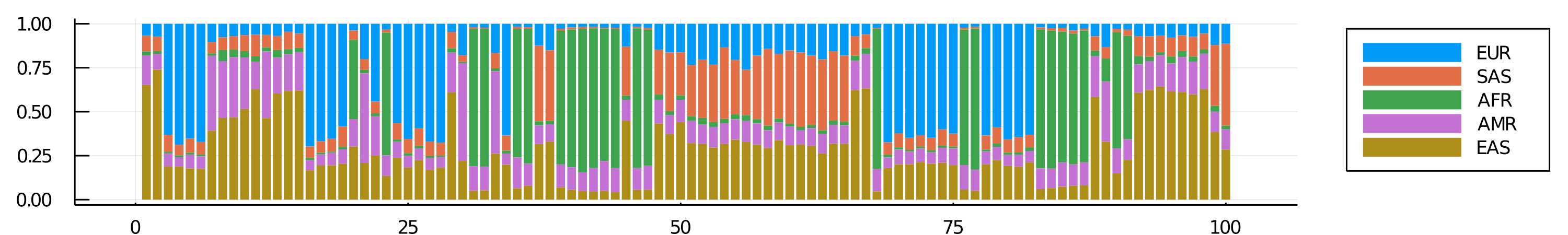

Local ancestry inference

Now we turn to local ancestry inference, or chromosome painting. We still need to process each sample's population origin as detailed in the top of this page. The only difference is now you must additionally supply a color gradient for different populations manually.

# We pick our colors here: https://mdigi.tools/color-shades/#008000.
continent = ["SAS", "EAS", "EUR", "AMR", "AFR"]
continent_colors = [colorant"#e6194B", colorant"#800000", colorant"#4363d8", colorant"#0000b3", colorant"#bfef45"]

# run MendelImpute to get local ancestries
tgtfile = "target.chr22.typedOnly.masked.vcf.gz"
reffile = "ref.chr22.maxd1000.excludeTarget.jlso"
Q, pop_colors = admixture_local(tgtfile, reffile, refID_to_superpopulation, 
    continent, continent_colors);

Number of threads = 1
Importing reference haplotype data...


Computing optimal haplotypes...100%|████████████████████| Time: 0:00:24
Phasing...100%|█████████████████████████████████████████| Time: 0:00:05


Total windows = 1634, averaging ~ 508 unique haplotypes per window.

Timings: 
    Data import                     = 8.32839 seconds
        import target data             = 1.71787 seconds
        import compressed haplotypes   = 6.61052 seconds
    Computing haplotype pair        = 24.912 seconds
        BLAS3 mul! to get M and N      = 1.27734 seconds per thread
        haplopair search               = 23.2227 seconds per thread
        initializing missing           = 0.136352 seconds per thread
        allocating and viewing         = 0.238768 seconds per thread
        index conversion               = 0.0202952 seconds per thread
    Phasing by win-win intersection = 5.7508 seconds
        Window-by-window intersection  = 0.88523 seconds per thread
        Breakpoint search              = 4.53825 seconds per thread
        Recording result               = 0.299743 seconds per thread
    Imputation                     = 0.172601 seconds
        Imputing missing               = 0.00086028 seconds
        Writing to file                = 0.171741 seconds

    Total time                      = 39.1647 seconds

Lets plot the local ancestries of

• Samples 1 (British)
• Sample 4 (Chinese)
• Sample 84 (Kenyan)

Their haplotypes occupy rows 1-2, 7-8, and 167-168 of Q, and their haplotype colors are stored in corresponding rows of pop_colors.

# sample index and axis labels
sample_idx = [1, 2, 7, 8, 167, 168]
sample_Q = Q[sample_idx, :]
sample_color = pop_colors[sample_idx, :]

# make plot
xnames = ["Sample 1 hap1", "Sample 1 hap2", "Sample 4 hap1", "Sample 4 hap2", "Sample 84 hap1", "Sample 84 hap2"]
ynames = ["SNP 1", "SNP 208k", "SNP 417k"]
local_plt = groupedbar(sample_Q, bar_position = :stack, bar_width=0.7, label=:none, 
    color=sample_color, xticks=(1:1:6, xnames), yticks=(0:0.5:1, ynames),
    ytickfont=font(12), xtickfont=font(12), xrotation=20, grid=false, 
    right_margin = 30Plots.mm, linecolor=:match)

# create a separate plot for legend
xlength = length(continent)
scatter!(local_plt, ones(xlength), collect(1:xlength), color=continent_colors, ytick=(1:xlength, continent), 
    xrange=(0.9, 1.1), xtick=false, label=:none, markersize=6, ytickfont=font(12),
    grid=false, framestyle=:grid, mirror=true, tick_direction=:out, markershape=:rect,
    inset = (1, bbox(-0.05, -0.1, 0.05, 1.1, :bottom, :right)), subplot = 2)

# save figure
# savefig(local_plt, "local_admixture.png")

Conclusion:

• We can visualize the linkage patterns for the 3 samples across their 6 haplotypes
• Sample 1 (British) is mostly European and admixed American, sample 2 (Chinese) is mainly South/East Asian, and sample 3 (Kenyan) is mainly African.

For more details, please refer to our paper, or file an issue on GitHub.