Iterative hard thresholding Tutorial
This notebook showcase a few examples of the software MendelIHT.jl.
#load necessary packages, install them if you don't have it
using MendelIHT
using SnpArrays
using DataFrames
using Distributions
using Random
using LinearAlgebra
using GLM
using DelimitedFiles
using Statistics
using BenchmarkTools
using Plots
What is IHT?
Iterative hard thresholding (IHT) is a sparse approximation method that performs variable selection and parameter estimation for high dimensional datasets. IHT returns a sparse model with prespecified $k \in \mathbb{Z}_+$ (or fewer) non-zero entries. In MendelIHT.j, the objective function is:
\begin{align} \text{maximize } & \quad L(\beta)\\ \text{subject to } & \quad ||\beta||_0 \le k \end{align}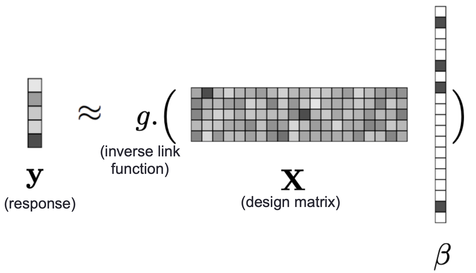
The objective is solved via projected gradient ascent: $$\beta_{n+1} = P_{S_k}(\beta_n + s_n \nabla L(\beta_n)),$$ where:
- $\nabla L(\beta)$ is the score (gradient) vector of loglikelihood
- $J(\beta)$ is the expected information (hessian) matrix
- $s = \frac{||\nabla L(\beta)||_2^2}{\nabla L(\beta)^tJ(\beta)\nabla L(\beta)}$ is the step size
- $P_{S_k}(v)$ projects vector $v$ to sparsity set $S_k$ by setting all but the top $k$ entries to 0.
See our paper for more details and computational tricks to do each of these efficiently.
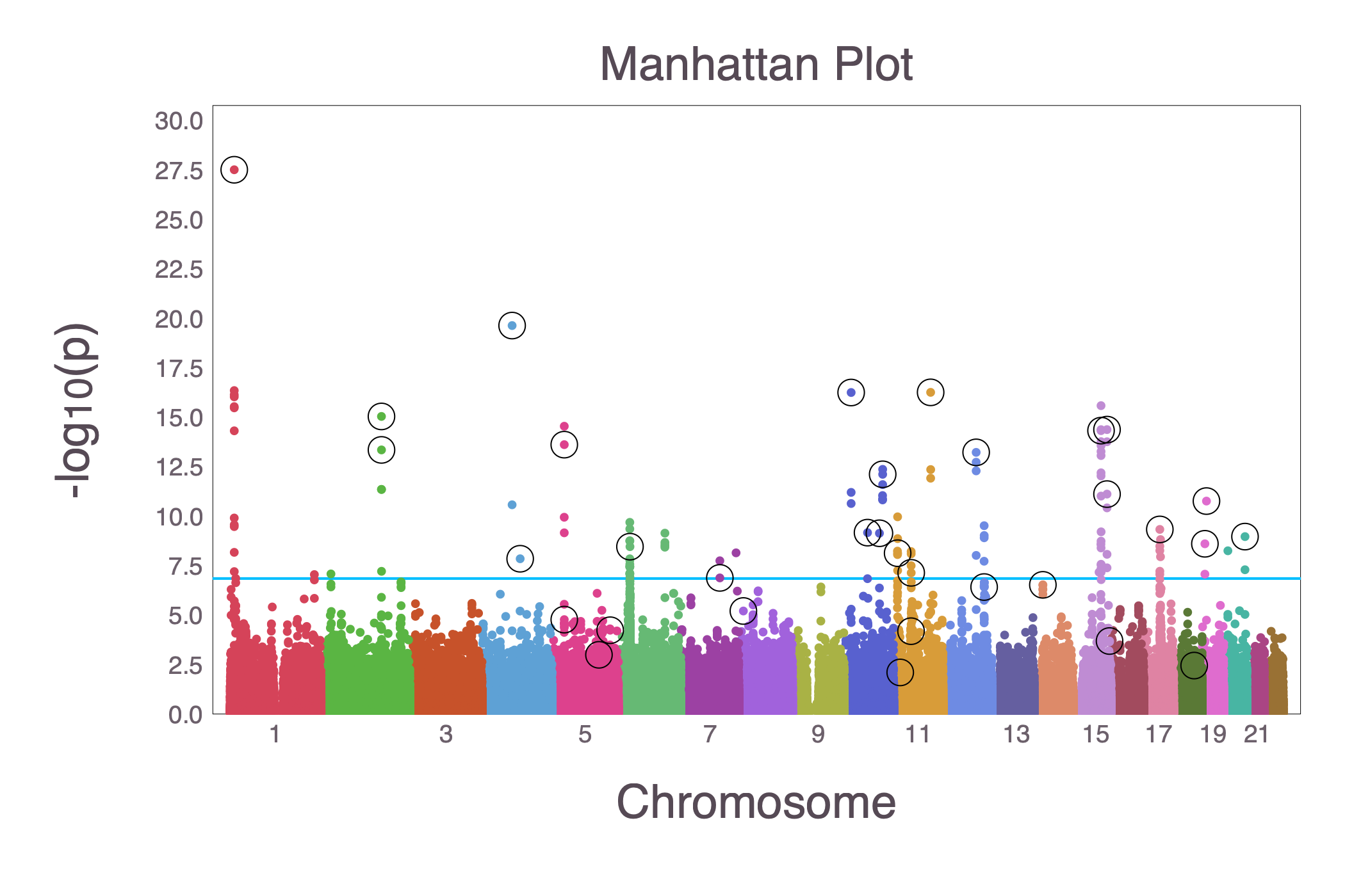
Example: IHT vs logistic GWAS on UK Biobank
- Data: ~200,000 samples and ~500,000 SNPs
- Ran 5-fold cross validated IHT for sparsity levels 1~50, distributed to 5 computers. Each completed with 24h. Total run time $<2$ days.
- Found 33 significant SNPs, plotted against traditional GWAS result using MendelPlots.jl:
Supported GLM models and Link functions
MendelIHT borrows distribution and link functions implementationed in GLM.jl and Distributions.jl.
| Distribution | Canonical Link | Status |
|---|---|---|
| Normal | IdentityLink | $\checkmark$ |
| Bernoulli | LogitLink | $\checkmark$ |
| Poisson | LogLink | $\checkmark$ |
| NegativeBinomial | LogLink | $\checkmark$ |
| Gamma | InverseLink | experimental |
| InverseGaussian | InverseSquareLink | experimental |
Examples of these distributions in their default value is visualized in this post.
Available link functions
CauchitLink
CloglogLink
IdentityLink
InverseLink
InverseSquareLink
LogitLink
LogLink
ProbitLink
SqrtLink
Note: Adding your favorite distribution only requires implementation of loglikelihood, score, and expected information!
Example 1: How to Import Data
Simulate example data (to be imported later)
First we simulate an example PLINK trio (.bim, .bed, .fam) and non-genetic covariates, then we illustrate how to import them. For genotype matrix simulation, we simulate under the model:
# rows and columns
n = 1000
p = 10000

#random seed
Random.seed!(2020)

# simulate random `.bed` file
x = simulate_random_snparray(n, p, "./data/tmp.bed")

# create accompanying `.bim`, `.fam` files (randomly generated)
make_bim_fam_files(x, ones(n), "./data/tmp")

# simulate non-genetic covariates (in this case, we include intercept and sex)
z = [ones(n, 1) rand(0:1, n)]
writedlm("./data/tmp_nongenetic_covariates.txt", z)
Reading Genotype data and Non-Genetic Covariates from disk
x = SnpArray("./data/tmp.bed")
z = readdlm("./data/tmp_nongenetic_covariates.txt")
Standardizing Non-Genetic Covariates.
We recommend standardizing all genetic and non-genetic covarariates (including binary and categorical), except for the intercept. This ensures equal penalization for all predictors. For genotype matrix, SnpBitMatrix efficiently achieves this standardization. For non-genetic covariates, we use the built-in function standardize!.
# SnpBitMatrix can automatically standardizes .bed file (without extra memory) and behaves like a matrix
xbm = SnpBitMatrix{Float64}(x, model=ADDITIVE_MODEL, center=true, scale=true);

# using view is important for correctness
standardize!(@view(z[:, 2:end]))
z
Example 2: Running IHT on Quantitative Traits
In this example, our model is simulated as:
$$y_i \sim \mathbf{x}_i^T\mathbf{\beta} + \epsilon_i$$$$x_{ij} \sim \rm Binomial(2, \rho_j)$$$$\rho_j \sim \rm Uniform(0, 0.5)$$$$\epsilon_i \sim \rm N(0, 1)$$$$\beta_i \sim \rm N(0, 1) \quad (\text{for 10 different } i)$$# Define model dimensions, true model size, distribution, and link functions
n = 1000
p = 10000
k = 10
dist = Normal
link = canonicallink(dist())
# set random seed for reproducibility
Random.seed!(2020)
# simulate SNP matrix, store the result in a file called tmp.bed
x = simulate_random_snparray(n, p, "./data/tmp.bed")
#construct the SnpBitMatrix type (needed for L0_reg() and simulate_random_response() below)
xbm = SnpBitMatrix{Float64}(x, model=ADDITIVE_MODEL, center=true, scale=true);
# intercept is the only nongenetic covariate
z = ones(n, 1)
# simulate response y, true model b, and the correct non-0 positions of b
y, true_b, correct_position = simulate_random_response(x, xbm, k, dist, link);
Step 1: Run q-fold cross validation to determine best model size
To run cv_iht, you must specify path and q, defined below:
path: all the model sizes you wish to test.q: number of disjoint partitions of your data.
By default, we partition the training/testing data randomly, but you can change this by inputing the fold vector as optional argument. In this example we tested $k = 5, 6, ..., 15$ across 3 fold cross validation. This is equivalent to running IHT across 30 different models, and hence, is ideal for parallel computing (which you specify by parallel=true).
path = collect(5:15)      # various sparsity levels to test (in this case 5 through 15)
q    = 3                  # number of fold cross validation

# Inputs: x, z, y = genotype matrix, other covariates, and response, 1 = group info (none)
@time mses = cv_iht(Normal(), IdentityLink(), x, z, y, 1, path, q, parallel=false);
plot(path, mses, label="Mean Squared Error", xlabel="Sparsity level",
        ylabel="Mean Squared Error", linewidth=5)
Step 2: Run IHT on full model for best estimated k
best_k = path[argmin(mses)]                                        # k = 7 minimizes MSE
result = L0_reg(x, xbm, z, y, 1, best_k, Normal(), IdentityLink()) # run IHT on full data
Check final model against simulation
Since all our data and model was simulated, we can see how well cv_iht combined with L0_reg estimated the true model. For this example, we find that IHT found every simulated predictor, with 0 false positives.
compare_model = DataFrame(
    true_β      = true_b[correct_position],
    estimated_β = result.beta[correct_position])
Conclusion: IHT found 7/10 true predictors, with superb parameter estimates. The remaining 3 predictors cannot be identified by IHT because they have very small effect sizes.
Example 3: Negative Binomial regression with group information
Now we show how to include group information to perform doubly sparse projections. This results in a model with at most $j$ groups where each group contains at most $k$ SNPs. This is useful for:
- Data with extensive LD blocks (i.e. correlated covariates)
- Prior knowledge on genes/pathways
Simulation: IHT on extensive LD blocks
In this example, we simulated:
- 10,000 SNPs, each belonging to 1 of 500 disjoint groups. Each group contains 20 SNPs
- $j = 5$ groups are each assigned $1,2,...,5$ causal SNPs with effect sizes randomly chosen from $\{−0.2,0.2\}$.
- Within group correlation: $\rho = 0.95$
We assume perfect group information. That is, the selected groups containing 1∼5 causative SNPs are assigned maximum within-group sparsity $\lambda_g = 1,2,...,5$. The remaining groups are assigned $\lambda_g = 1$ (i.e. only 1 active predictor are allowed).
# define problem size
n = 1000
p = 10000
dist = NegativeBinomial
link = LogLink()
block_size = 20                  #simulation parameter
num_blocks = Int(p / block_size) #simulation parameter

# set seed
Random.seed!(2020)

# assign group membership
membership = collect(1:num_blocks)
g = zeros(Int64, p + 1)
for i in 1:length(membership)
    for j in 1:block_size
        cur_row = block_size * (i - 1) + j
        g[block_size*(i - 1) + j] = membership[i]
    end
end
g[end] = membership[end]

#simulate correlated snparray
x = simulate_correlated_snparray(n, p, "./data/tmp2.bed", prob=0.95)
z = ones(n, 1) # the intercept
x_float = convert(Matrix{Float64}, x, model=ADDITIVE_MODEL, center=true, scale=true)

#simulate true model, where 5 groups each with 1~5 snps contribute
true_b = zeros(p)
true_groups = randperm(num_blocks)[1:5]
sort!(true_groups)
within_group = [randperm(block_size)[1:1], randperm(block_size)[1:2],
                randperm(block_size)[1:3], randperm(block_size)[1:4],
                randperm(block_size)[1:5]]
correct_position = zeros(Int64, 15)
for i in 1:5
    cur_group = block_size * (true_groups[i] - 1)
    cur_group_snps = cur_group .+ within_group[i]
    start, last = Int(i*(i-1)/2 + 1), Int(i*(i+1)/2)
    correct_position[start:last] .= cur_group_snps
end
for i in 1:15
    true_b[correct_position[i]] = rand(-1:2:1) * 0.2
end
sort!(correct_position)

# simulate phenotype
r = 10 #nuisance parameter
μ = GLM.linkinv.(link, x_float * true_b)
clamp!(μ, -20, 20)
prob = 1 ./ (1 .+ μ ./ r)
y = [rand(dist(r, i)) for i in prob] #number of failures before r success occurs
y = Float64.(y);
IHT without group information
# x_float = genotype matrix in floating point numbers
# z       = other covariates
# y       = response vector

j = 1      # 1 active group = entire dataset
k = 15     # 15 active predictors
ungrouped_IHT = L0_reg(x_float, z, y, j, k, NegativeBinomial(), LogLink())
IHT with group information
# x_float = genotype matrix in floating point numbers
# z       = other covariates
# y       = response vector
# g       = group membership vector (simulated above)

j = 5                           # maximum number of active groups
dist = NegativeBinomial()       # distribution
link = LogLink()                # link function

# within-group sparsity for each group
max_group_snps = ones(Int, num_blocks)
max_group_snps[true_groups] .= collect(1:5)

# run grouped IHT
grouped_IHT = L0_reg(x_float, z, y, j, max_group_snps, NegativeBinomial(), LogLink(), group=g)
Check variable selection against true data
compare_model = DataFrame(
    correct_positions = correct_position,
    ungrouped_IHT_positions = findall(!iszero, ungrouped_IHT.beta),
    grouped_IHT_positions = findall(!iszero, grouped_IHT.beta))
Check estimated parameters against true data
correct_position = findall(!iszero, true_b)
compare_model = DataFrame(
    position = correct_position,
    correct_β = true_b[correct_position],
    ungrouped_IHT_β = ungrouped_IHT.beta[correct_position],
    grouped_IHT_β = grouped_IHT.beta[correct_position])
Conclusion: by asking for "top entries" in each group, we (somewhat) disentangle the correlation structure in our data and achieved better model selection!
More examples:
Please visit our documentation.
Other functionalities
- Built-in support for PLINK binary files via SnpArrays.jl and VCF files via VCFTools.jl.
- Out-of-the-box parallel computing routines for
q-foldcross-validation. - Fits a variety of generalized linear models with any choice of link function.
- Computation directly on raw genotype files.
- Efficient handlings for non-genetic covariates.
- Optional acceleration (debias) step to dramatically improve speed.
- Ability to explicitly incorporate weights for predictors.
- Ability to enforce within and between group sparsity.
- Naive genotype imputation.
- Estimates nuisance parameter for negative binomial regression using Newton or MM algorithm.