Heritability analysis and testing SNP association using maximum likelihoods of variance component models
Lange Symposium
Juhyun Kim, juhkim111@ucla.edu
Department of Biostatistics, UCLA
Feb 22, 2020
Machine information:
versioninfo()
VarianceComponentModels.jl
VarianceComponentModels.jl is a package that resides in OpenMendel ecosystem. It implements computation routines for fitting and testing variance component model of form
$$\text{vec}(Y) \sim \text{Normal}(XB, \Sigma_1 \otimes V_1 + \cdots + \Sigma_m \otimes V_m)$$
where $\otimes$ is the Kronecker product.
In this model, data is represented by
Y:n x dresponse matrixX:n x pcovariate matrixV=(V1,...,Vm): a tuple ofmn x ncovariance matrices
and parameters are
B:p x dmean parameter matrixΣ=(Σ1,...,Σm): a tuple ofmd x dvariance components.
Package Features
- Maximum likelihood estimation (MLE) and restricted maximum likelihood estimation (REML) of mean parameters $B$ and variance component parameters $Σ$
- Allow constraints in the mean parameters $B$
- Choice of optimization algorithms: Fisher scoring and minorization-maximization algorithm
- Heritability analysis in genetics
Heritability Analysis
Variance component estimation can be used to estimate heritability of a quantitative trait.
Data files
For this analysis, we use a sample data set EUR_subset from SnpArrays.jl. This data set is available in the data folder of the package.
using SnpArrays
datapath = normpath(SnpArrays.datadir())
EUR_subset.bed, EUR_subset.bim, and EUR_subset.fam is a set of Plink files in binary format.
using Glob
readdir(glob"EUR_subset.*", datapath)
Read in binary SNP data
We use the SnpArrays.jl package to read in binary SNP data and compute the empirical kinship matrix.
# read in genotype data from Plink binary file
const EUR_subset = SnpArray(SnpArrays.datadir("EUR_subset.bed"))
EUR_subset
EUR_subset contains 379 individuals and 54,051 SNPs. There is no missing genotype in EUR_subset.
Minor allele frequencies (MAF) for each SNP:
maf_EUR = maf(EUR_subset)
Histogram of minor allele frequency:
## generate a histogram of MAF
# using Plots, PyPlot
# gr(size=(600, 500), html_output_format=:png)
# hist_maf = histogram(maf_EUR, xlab = "Minor Allele Frequency (MAF)",
#                    ylab = "Number of SNPs", label="")
# png(hist_maf, "hist_MAF.png")
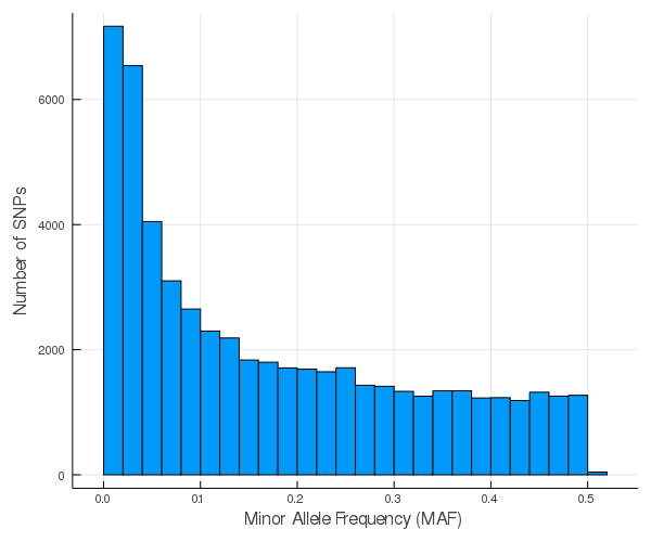
Note that about 29% of SNPs are rare variants (MAF < 0.05).
count(!iszero, maf_EUR .< 0.05) / length(maf_EUR)
Empirical kinship matrix
For a measure of relatedness, we compute empirical kinship matrix based on all SNPs by the genetic relation matrix (GRM). If there are missing genotypes, they are imputed on the fly by drawing according to the minor allele frequencies.
Kinship coefficients summarize genetic similarity between pairs of individuals. To estimate kinship coefficient $\Phi_{ij}$ between individuals $i$ and $j$ using GRM:
$$\widehat{\Phi}_{GRMij} = \frac{1}{2S} \sum_{k=1}^S \frac{(G_{ik}-2p_k)(G_{jk}-2p_k)}{2p_k(1-p_k)},$$
where
- $S$: number of SNPs in this set
- $p_k$: minor allele frequency of SNP $k$
- $G_{ik} \in \{0,1,2\}$: number of copies of minor alleles at the $k$-th SNP of the $i$-th individual
## GRM using SNPs with maf > 0.01 (default)
Φgrm = grm(EUR_subset; method = :GRM) # classical genetic relationship matrix
# Φgrm = grm(EUR_subset; method = :MoM) # method of moment method
# Φgrm = grm(EUR_subset; method = :Robust) # robust method
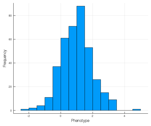
Simulating phenotypes
We simulate phenotype vector from
$$\mathbf{y} \sim \text{Normal}(\mathbf{1}, 0.1 \widehat{\Phi}_{GRM} + 0.9 \mathbf{I})$$
where $\widehat{\Phi}_{GRM}$ is the estimated empirical kinship matrix Φgrm.
The data should be available in pheno.txt.
## simulate `pheno.txt`
# using LinearAlgebra, DelimitedFiles
# Random.seed!(1234)
# Ω = 0.1 * Φgrm + 0.9 * Matrix(1.0*I, nobs, nobs)
# Ωchol = cholesky(Symmetric(Ω))
# y = ones(nobs) + Ωchol.L * randn(nobs)
# writedlm("pheno.txt", y)
Phenotypes
Read in the phenotype data and plot a histogram.
using DelimitedFiles
pheno = readdlm("pheno.txt")
Histogram of phenotype values:
## generate histogram of phenotype values
#hist_pheno = histogram(pheno, xlab="Phenotype", ylab="Frequency", label="")
#png(hist_pheno, "hist_pheno.png")
Pre-processing data for heritability analysis
To prepare variance component model fitting, we form an instance of VarianceComponentVariate. The two covariance matrices are $(2\Phi, I)$.
using VarianceComponentModels, LinearAlgebra
# no. of observations
nobs = size(pheno, 1)

# form data as VarianceComponentVariate
X = ones(nobs)
EURdata = VarianceComponentVariate(pheno, X, (2Φgrm, Matrix(1.0I, nobs, nobs)))
fieldnames(typeof(EURdata))
EURdata
Heritability of single trait
Before fitting the variance component model, we pre-compute the eigen-decomposition of $2\Phi_{\text{GRM}}$, the rotated responses, and the constant part in log-likelihood, and store them as a TwoVarCompVariateRotate instance, which is re-used in various variane component estimation procedures.
We use Fisher scoring algorithm to fit variance component model for our trait.
# pre-compute eigen-decomposition
@time EURdata_rotated = TwoVarCompVariateRotate(EURdata)
fieldnames(typeof(EURdata_rotated))

# form data set for trait
trait_data = TwoVarCompVariateRotate(EURdata_rotated.Yrot,
    EURdata_rotated.Xrot, EURdata_rotated.eigval, EURdata_rotated.eigvec,
    EURdata_rotated.logdetV2)

# initialize model parameters
trait_model = VarianceComponentModel(trait_data)

# estimate variance components
_, _, _, Σcov, = mle_fs!(trait_model, trait_data; solver=:Ipopt, verbose=false)
σ2a = trait_model.Σ[1][1] # additive genetic variance
σ2e = trait_model.Σ[2][1] # environmental variance
@show σ2a, σ2e
Additive genetic variance:
σ2a
Environmental/non-genetic variance:
σ2e
# heritability and its standard error from single trait analysis
h, hse = heritability(trait_model.Σ, Σcov)


[h[1], hse[1]]
We can also run MM algorithm.
trait_model = VarianceComponentModel(trait_data)
@time _, _, _, Σcov, = mle_mm!(trait_model, trait_data; verbose=false)
σ2a = trait_model.Σ[1][1]
σ2e = trait_model.Σ[2][1]
@show σ2a, σ2e
Heritability and its standard error.
h, hse = heritability(trait_model.Σ, Σcov)
[h[1], hse[1]]
Multivariate trait analysis
For the joint analysis of multiple traits, go to VarianceComponentModels documentation.
Exercise
Repeat the above analysis computing the empirical kinship matrix using the method of moment method or the robust method. See SnpArrays.jl documentation.
# Φgrm = grm(EUR_subset; method = )
Testing SNP association using maximum likelihoods of variance component models
credit: Heritability tutorial by Sarah Ji, Janet Sinsheimer and Hua Zhou
Suppose we want to see a particular SNP has an effect on a given phenotype after accounting for relatedness among individuals. Here we fit variance component model with a single SNP s as fixed effect.
$$\hspace{5em} \mathbf{y} = \mathbf{X}\mathbf{\beta} + \mathbf{G}_s \gamma + \mathbf{g} + \mathbf{\epsilon} \hspace{5em} (1)$$
\begin{equation} \begin{array}{ll} \mathbf{g} \sim N(\mathbf{0}, \sigma_g^2\mathbf{\Phi}) \\ \mathbf{\epsilon} \sim N(\mathbf{0}, \sigma_e^2\mathbf{I}) \end{array} \end{equation}
where
- $\mathbf{y}$: phenotype
and
- Fixed effects:
- $\mathbf{X}$: matrix of covariates including intercept
- $\beta$: vector of covariate effects, including intercept
- $\mathbf{G}_s$: genotype of SNP s
- $\gamma$: (scalar) association parameter of interest, measuring the effect of genotype on phenotype
- Random effects:
- $\mathbf{g}$: random vector of polygenic effects with $\mathbf{g} \sim N(\mathbf{0}, \sigma_g^2 \mathbf{\Phi})$
- $\sigma_g^2$: additive genetic variance
- $\mathbf{\Phi}$: matrix of pairwise measures of genetic relatedness
- $\epsilon$: random vector with $\epsilon \sim N(\mathbf{0}, \sigma_e^2\mathbf{I})$
- $\sigma_e^2$: non-genetic variance due to non-genetic effects assumed to be acting independently on individuals
- $\mathbf{g}$: random vector of polygenic effects with $\mathbf{g} \sim N(\mathbf{0}, \sigma_g^2 \mathbf{\Phi})$
To test whether SNP s is associated with phenotype, we fit two models. First consider the model without SNP s as fixed effects (aka null model):
$$\hspace{5em} \mathbf{y} = \mathbf{X}\mathbf{\beta} + \mathbf{g} + \mathbf{\epsilon} \hspace{5em} (2)$$
and the model with SNP s as fixed effects (1). Then we can compare the log likelihood to see if there is improvement in the model fit with inclusion of the SNP of interest.
Fit the null model
using VarianceComponentModels
# null data model has two variance components but no SNP fixed effects
# form data as VarianceComponentVariate matrix
X = ones(nobs)
nulldata = VarianceComponentVariate(pheno, X, (2Φgrm, Matrix(1.0I, nobs, nobs)))
nullmodel = VarianceComponentModel(nulldata)
@time nulllogl, nullmodel, = fit_mle!(nullmodel, nulldata; algo=:FS)
The null model log-likelihood (no SNP effects)
nulllogl
The null model mean effects (a grand mean)
nullmodel.B
The null model additive genetic variance
nullmodel.Σ[1]
The null model environmental variance
nullmodel.Σ[2]
Fit the alternative model
snp_vec = convert(Vector{Float64}, EUR_subset[:, 10])
Xalt = [ones(nobs) snp_vec]
altdata = VarianceComponentVariate(pheno, Xalt, (2Φgrm, Matrix(1.0I, nobs, nobs)))
altmodel = VarianceComponentModel(altdata)
@time altlogl, altmodel, = fit_mle!(altmodel, altdata; algo=:FS)
The alternative model log-likelihood:
altlogl
The alternative model mean effects (a grand mean)
altmodel.B
The alternative model additive genetic variance
altmodel.Σ[1]
The alternative model environmental variance
altmodel.Σ[2]
Likelihood ratio test
We use likelihood ratio test (LRT) to test the goodness-of-fit between two models.
Our likelihood ratio test statistic is 1.786 (distributed chi-squared), with one degree of freedom.
using Distributions
LRT = 2(altlogl - nulllogl)
The associated p-value:
pval = ccdf(Chisq(1), LRT)
We see that adding this SNP as a covariate to the model does not fit significantly better than the null model. In other words, the SNP does not explain more of the variation in our trait.
Exercise
Use minorization-maximization algorithm (algo=:MM) to find MLEs of both null model and alternative model. Then conduct the likelihood ratio test.